
Sections:
- 1. Introduction
- 2. Data Description
- 3. Fully Convolutional Model
- 4. Densenet Based Classifier
- References
Introduction:
Astronomy has historically been one of the most data intensive fields & a major chunk of this data is collected as images collected by a number of telescopes - terrestrial as well as in space. A BIG data-project which aims to collate this data from various sources to form a coherent picture of the universe is Sloan Digital Sky Survey.
To quote the project website :
A citizen science project called Galaxy zoo was launched in 2007, through this project thousands of volunteers classified 100k+ images of galaxies. A flow-chart of questions asked to volunteers shown on the project website is as follows.

Data Description:
The dataset consists of 100k+ jpeg images and the corresponding score vector for each image. The score vector has 37 values where each value represents the weighted score from volunteers in the project.
The important point to remember is that the scores aren’t probability score per se. They are weighted scores & so they vary from 0 to 1 but all sub scores for a question don’t necessarily sum up to 1 as a rule.
Each image is of size 424x424x3 & each value is between 0-255. A good practice is to rescale the data. In our experiments, we normalize the images by calculating \(\mu_{channel}\) and \(\sigma_{channel}\) over the full dataset and then normalizing each channel using their correspodning \(\mu\) and \(\sigma\). The channels & cell values do not represent the physical aspect of data collection, but are standardized to the accepted image formats between 0-255 and so the normalization is more of a hack for better gradient updates and not adomain knowledge based modification.
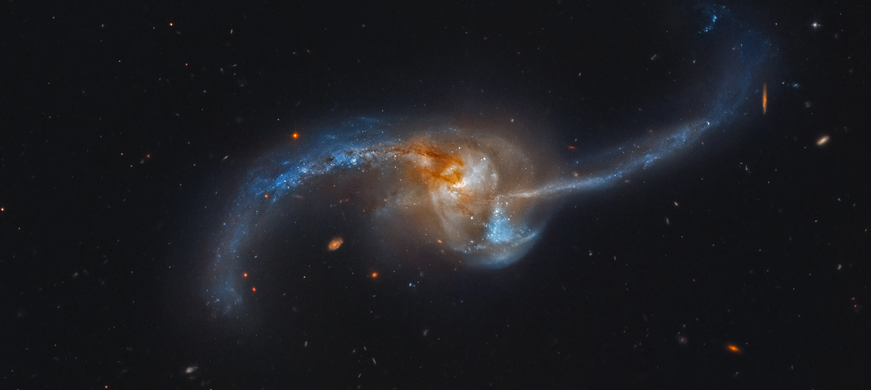
A few sample images from the dataset:

These images are read in as numpy arrays in python with the following representation:

Fully Convolutional Classifier:
A convolutional network takes in your image array as input extracts features from this array which best represents the task at hand & then gives out a classification/regression output. Standard classification models use one-vs-rest scheme to represent output for an elegant representation of the classification task. In this form, the correct class is assigned 1 while other possible classes in the dataset are assigned 0. The output vector is of length c, where c is total number of classes in the dataset.
In the Galaxy Morphology classification task, we use standard .jpeg images to learn the shape attributes as a vector of length 37 which describes its properties. We set it up as a regression task in this case, since our ground truth is a weighted version of votes gathered from volunteers.
The model takes in a normalized array representing input image. This array passes through the following layers stacked after each other:
-
Convolutional layer : It consists of a set of learnt features. In terms of standard modeling terminology, the features that a model uses are usually handcrafted i.e. some form of transformations of the raw input data. In images, the kernels that form the convolutional layer are expected to learn optimal features for the task at hand, instead of features crafted by a domain expert. Since the output from this convolutional layer is learnt w.r.t output, the features being generated at each step should ideally be the optimal representation of input provided at that step.
-
Pooling layer : The pooling layer reduce size of incoming representation by selecting from a set of appropriate downsampling functions. The
max-poolinglayer chooses maximum from a given volume of array as an appropriate representation of the focus. Similarly,average-poolingtakes average of the volume. -
Activation : Activation functions are used to introduce non-linearity in the model. This layer applies a given function to each element of input array. Standard activation functions used in models are ‘relu’, ‘softmax’, ‘sigmoid’, ‘tanh’ etc.
-
Dropout : Dropout is a technique developed to reduce overfitting in deep neural networks. The effect of adding this layer is equal to setting activations for a fraction of neurons to
zeroduring training time & during test time, using that fraction as weighted average for the weights being used i.e. during training time, a particualr unit ‘ll is present with probabilityp& during prediction, the weights learnt for this particular unit are multiplied byp. Below, (a) represents a standard net with no dropout and (b) represents dropout applied to the same network. After droput, each layer has some fraction of activations set to zero, thus effectively reducing the impact of that neuron in the final model.
-
Batch normalization : A major problem encountered while training neural networks is the variation in distribution of input values to successive layers. Due to this, a large number of updates with an extremely small update rate are required. By using batch-normalization, we normalize the input at each layer to μx = 0 & σx = 1. Effectively, we end up with higher learning rates giving the same results. Effectively,
Batchnormalizationimplements the following transform :
Here, μX and σX are calculated and applied channelwise. Hence, the normalization is effectively channelwise normalization of the representation generated by the previous layer and being provided to the next layer.
Setup :
The layers in a neural network are stacked one afer the other to be used as a module & we experiment with different network structures starting with some well tested & prevalent ones to some recently pulished. The last few layers are Dense layers, i.e. they are fully connected layers and their final output is compared with the expected output to calculate error value for the observation in focus. This error is back-propagated to give higher or lower importance to the learnt features of convolutional layers & nodes of dense layers. With each bacward pass of these error values, the expectation is that given enough data, our network structure learns optimal features for solving the problem at hand.
In our setup, the intermediate features are extracted successeivel from the raw galaxy image & then the corresponding regression is done to match human generated score for the the same image. This score is a vector of 37 values, each representing a physical aspect of the galaxy, termed as galaxy morphology.
References :
-
Dropout : Dropout: A Simple Way to Prevent Neural Networks from Overfitting
-
BatchNormalization : Batch Normalization: Accelerating Deep Network Training by Reducing Internal Covariate Shift